Introduction
A fundamental part of experimental economic research is writing pre-analysis plans, which serve as a commitment device for the hypotheses we wish to test and the number of participants we aim to recruit. In outlining the specific questions we are seeking to answer with a specific sample size, we can reassure future readers that the findings we describe are not a coincidence which we stumbled upon as we analyzed our data, lending increased credibility to the experimental results. The following sections describe one particular (preliminary) exercise conducted in the pre-analysis plan for a working paper of mine, Campos et al (2019).
Our project is a natural follow-up to a submitted project of mine, Goette et al (2019), in which we derive and test comparative static predictions of the KR model in the endowment effect context with heterogeneous gain-loss types. Specifically, we consider two types of agents: loss averse and gain loving. Loss averse individuals, roughly speaking, are defined as those who would accept a 50-50 gamble of +$10+x, -$10 for x>0; intuitively, these agents dislike losses around a reference point (assumed 0 here) more than equal sized gains, and would thus need to be compensated with a bigger payoff to accept the possibility of a $10 loss. The larger the x before they accept, the more loss averse. Gain lovers, in the same rough terms, would actually accept gambles where x<0 because, intuitively, they enjoy the surprise of the lottery, and enjoy gains above the reference point more than commensurate losses.
In Goette et al (2019), we show that lab participants previously measured to be gain loving vs loss averse respond quite differently to a treatment that is commonly used to test the KR model. Importantly, prior analysis of these types has tended to ignore the heterogeneity and test the treatment assuming that people are loss averse on average. Although this is empirically true, the 15-30% of gain lovers have an outsized role in aggregate treatment effects, which we uncover in our paper. The pre-analysis exercise described below applies this same experimental framework to a different domain, to explore whether these gain-loss classifications predict behavior in the real effort setting.
Power Analysis Overview and Code
Before we run our experiments in this new domain, we want to be sure that the theoretical predictions yield interesting, testable implications that can be measured with reasonable sample sizes. To get a feel for this, we run simulations on bootstrapped data, allowing us to recover expected treatment effect sizes under heterogeneous populations. From the data in Goette et al (2019), we obtain a distribution of gain-loss attitudes measured in a lab population — which we assume to be representative despite the domain change. From Augenblick and Rabin (2018), we obtain MLE estimates of the cost of effort function under a particular functional form assumption, using the same task as we will in this experiment (see Table 1 for parameter estimates). With these distributions of parameters in hand, we have all the requisite information to generate simulated behavior under the KR model, specifically the CPE assumption.
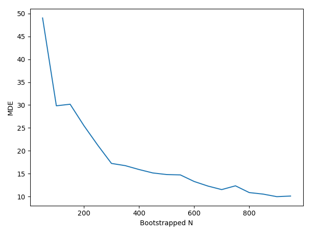
For a range of sample sizes, we bootstrap from these distributions and generate simulated behavior, which we subsequently feed into our regression of interest. For each of the sample sizes we consider, we store the estimated regression coefficient as well as the minimum detectable effect size (approximated by 2.8*SE(coef) as in Page 16 of these JPAL slides), which we ultimately plot against the bootstrapped sample. This plot helps inform us of what types of effect sizes we can reject at different sample sizes; by examining our simulated effect sizes, we are able to map the results and determine the number of participants we require.
Note that there are a number of simplifications in this code, and the final sample size will be determined using a slightly different procedure. Specifically, the analysis herein assumes we know the gain-loss value (lambda), whereas in our study, we will estimate it from experimental data. Because this introduces additional noise, we expect attenuation bias in our parameter estimates. This, and other details that were skipped over, will be discussed at length in the pre analysis plan; as soon as it is posted, I will link to it.
This Python code implements the aforementioned procedure, generating a preliminary MDE curve.
'''
Code Overview: Using data from Goette et al (2019) and Augenblick and Rabin (2019),
we bootstrap a distribution of gain-loss and cost of effort function parameters to
conduct a power analysis on our experimental hypothesis. Ultimately, we hope to
determine the requisite sample size to test our coefficient of interest with 80%
power at the 5% two-sided level.

Author: Alex Kellogg
'''

#Import required modules for the ensuing analysis
import numpy as np
import pandas as pd
import matplotlib.pyplot as plt
import statsmodels.formula.api as sm

'''
We assume the distribution of gain-loss attitudes follows that in Goette et al (2019)
for  this analysis. This data was estimated via MLE in a prior project, and is
generally representative of the experimentally measured distributions throughout the
literature.
'''

#Read in the relevant columns from full Goette et al (2019) lab data
ggks_dataset=pd.read_csv("dir/pooled_data.csv", usecols=['stage1_lambda','structla'])

'''
Because our task is adopted from Augenblick and Rabin (2019), who have prior
MLE estimates of the cost of effort function given their assumed functional
form, we opt to model effort costs in the form below. This allows us to introduce
heterogeneity in a rigorous manner to both cost of effort and gain-loss attitudes.
'''

def cost_of_effort(e, c_slope, c_curv):
    '''
    :param e: Effort, or the number of tasks (b/w 0 and 100).
    :param c_slope: Slope parameter, normalizing tasks to dollar costs.
    :param c_curv: Curvature parameter determining convexity of cost function.
    :return: (Negative of) Utility from completing e tasks.
    '''
    return (1/(c_slope*c_curv))*((e+10)**c_curv)

'''
We assume individual utility follows KR06 CPE, so that there is no gains/losses
in the effort domain as the number of tasks are preselected, but uncertainty
in wages yields gain-loss comparisons against reference points. Specifically,
each feasible ex-ante outcome is compared to the others, weighted by their a-priori
likelihood.

'''
def cpe_utils(e, c_slope, c_curv, wage, fixed, lam):
    '''

    :param e: The number of tasks considered.
    :param c_slope: Slope parameter, normalizing tasks to dollar costs.
    :param c_curv: Curvature parameter determining convexity of cost function.
    :param wage: Piece-rate (per task) rate of payment.
    :param fixed: Outside option, which is earned regardless of effort with 50%.
    :param lam: Gain-loss Attitude parameter, lam>1 implies loss aversion.
    :return: KR06 CPE utility of working e tasks given the preference parameters and wage rates.
    '''

    return 0.5*e*wage+0.5*fixed-0.5*(lam-1)*abs(fixed-wage*e)-cost_of_effort(e,c_slope,c_curv)

'''
Unfortunately, there is no closed form solution to the problem of optimal effort with
fixed vs piece-rate wages. Thus, to determine the optimal utility given the parameters,
we conduct a grid search over the possible values of effort, which can range between 0
and 100 tasks. The alternative to a grid search is a series of elseif conditions to
determine how the Marginal Benefit and Marginal Cost curves relate to each other, but
the number of checks is extensive and thus the computational cost of the grid search
outweighs the speed but increased error rate of the checklist approach.
'''

#Loop over the possible task choices for the agent given the parameters, and store the optimal
def optimal_effort_solver(c_slope, c_curv, wage, fixed, lam):
    '''
    :param c_slope: Slope parameter, normalizing tasks to dollar costs.
    :param c_curv: Curvature parameter determining convexity of cost function.
    :param wage: Piece-rate (per task) rate of payment.
    :param fixed: Outside option, which is earned regardless of effort with 50%.
    :param lam: Gain-loss Attitude parameter, lam>1 implies loss aversion.
    :return: The number of tasks that yields maximum CPE Utils.
    '''
    effort_space = np.arange(0, 100.1, 0.1)
    utils_vec=[]
    for a in effort_space:
        tempU= cpe_utils(a, c_slope, c_curv, wage, fixed, lam)
        utils_vec.append(tempU)
    utils_vec = np.asarray(utils_vec)
    max_ind = np.argmax(utils_vec)
    return effort_space[max_ind]

#Define a function the computes the between subjects interaction regression.
def treatment_effect_bootstrapped_between_lambda(data):
    '''
    :param data: Dataframe containing the relevant variables for the regression specification.
    :return: Regression Result.
    '''

    #generate a new effort variable that captures only the relevant effort given treatment
    data['Effort']=data['Treatment']*data['Effort_Choice_Hi_Fixed']+(1-data['Treatment'])*data['Effort_Choice_Low_Fixed']

    data['Interaction']=data['Treatment']*data['Lambda']

    result = sm.ols(formula="Effort ~Treatment+Lambda+Interaction", data=data).fit()
    return result

#Create a function to plot the Minimum Detectable Effect size
def mde_plotter(n_list, mde_list):
    '''

    :param n_list: np.array of the sample sizes we considered in the MDE analysis.
    :param mde_list: List of the mde's generated in the analysis.
    :return: Plot the MDE for each sample size.
    '''
    mde_list=np.asarray(mde_list)
    plt.plot(n_list,mde_list)
    plt.xlabel('Bootstrapped N')
    plt.ylabel('MDE')
    plt.show()

#Set up the parameters for our MDE analysis loop.
bootstrap_N_list=np.arange(50,1000,50)
bootstrap_MDE=[]
bootstrap_te=[]

'''
Iterate over each of the sample sizes and compute the MDE at that sample size.
To do so, we will sample bootstrap_N gain-loss, cost slope (constant here),
and cost curvature parameters from their assumed distributions, based on prior work.
We take this sample to be our experimental subject pool, and simulate the decisions
we would observe from these subjects if they decided according to KR CPE. We then run
our interaction specification on our full sample and record the parameter estimate for
coefficient of interest, as well as the mde, which is approximated by 2.8*SE(beta).
'''
for bootstrap_N in bootstrap_N_list:
    #sample lambdas with replacement from the empirical distribution to create our own distribution
    id = np.random.choice(np.arange(len(ggks_dataset.stage1_lambda)), bootstrap_N, replace=True)
    sampled_lambda = np.asarray(ggks_dataset.stage1_lambda[id])
    sampled_structla = np.asarray(ggks_dataset.structla[id])

    #for the cost function, we borrow numbers from Table 1 (pg 29) in AR19 assuming the large sample properties of MLE.
    #that is, we take the estimated MLE and associated sd to be distributed normally, and draw from them.
    # cost slope represents phi in the AR cost function.
    cost_slope = [724] * bootstrap_N
    # cost curvature represents gamma.
    cost_curvature = np.random.normal(2.138, 0.692, size=bootstrap_N)

    #To cut the computation in half, we solve for the optimal effort in the condition for which this simulant will ultimately wind up.
#This is a between subjects regression, so it is unaffected.
    treatment_assignment=np.random.randint(2, size=bootstrap_N)

    effort_choices_l=[]
    effort_choices_h=[]
    for i in np.arange(0,bootstrap_N):
        if treatment_assignment[i]==0:
            effort_choices_l.append(optimal_effort_solver(cost_slope[i], cost_curvature[i], 0.25, 5, sampled_lambda[i]))
            effort_choices_h.append(-1)
        else:
            effort_choices_l.append(-1)
            effort_choices_h.append(optimal_effort_solver(cost_slope[i], cost_curvature[i],0.25,20,sampled_lambda[i]))

    #Define the dataframe to feed into the regression function.
    df_cols={
        'Effort_Choice_Low_Fixed':list(map(float, np.asarray(effort_choices_l))),
        'Effort_Choice_Hi_Fixed':list(map(float, np.asarray(effort_choices_h))),
        'Lambda': sampled_lambda,
        'Structla': sampled_structla,
        'Cost_Slope': cost_slope,
        'Cost_Curvature': cost_curvature,
        'Treatment': treatment_assignment
    }
    bootstapped_data = pd.DataFrame(df_cols)

    reg_results=treatment_effect_bootstrapped_between_lambda(bootstapped_data)
    bootstrap_MDE.append(reg_results.bse[3]*2.8)
    bootstrap_te.append(reg_results.params[3])

#plot the MDE curve
mde_plotter(bootstrap_N_list,bootstrap_MDE)
The resulting plot is displayed below. Our median effect size is roughly 15 tasks in this particular simulation, which would suggest a sample of about 400 to be sufficient.
Sources:
Augenblick, Ned and Matthew Rabin (2018). “An Experiment on Time Preference and Misprediction in Unpleasant Tasks”.
Goette, Lorenz, Thomas Graeber, Alexandre Kellogg, and Charles Sprenger (2018). “Het- erogeneity of Gain-Loss Attitudes and Expectations-Based Reference Points”.
Kőszegi, Botond and Matthew Rabin (2006). “A model of reference-dependent preferences”. In: The Quarterly Journal of Economics, pp. 1133–1165.
Kőszegi, Botond and Matthew Rabin (2007). “Reference-Dependent Risk Attitudes.” In: American Economic Review (4): 1047–73.