Maximum Simulated Likelihood (R)

Introduction

For an existing project, my coauthors and I use a number of statistical tools in conjunction with a structural model in order to recover preference parameters from experimental data. As described in extensive detail in the draft, we have designed a two-stage experiment in the classic endowment effect framework in an attempt to test the comparative statics of the KR model; our primary contribution is a theoretical and empirical demonstration that accounting for heterogeneity in individual gain-loss attitudes is crucial for generating/recovering predictions in this paradigm. In order to convincingly demonstrate this, we use our first stage experimental data to estimate gain-loss attitudes, from which we generate sharp, testable predictions that form our second stage hypothesis.

As the measurement of gain-loss attitudes is fundamental to our hypothesis, we experiment with a number of methods. Originally, we opted for a standard MLE procedure relying on random utility methods and our structural model. However, these estimates did not directly allow us to speak about the core heterogeneity in which we were interested. Because of this, we adapted our estimation procedure to a similar methodology more suited to measuring distributions: mixed logit. The key difference in this framework is that we assume our central parameter is normally distributed, with unobservable, individual-level noise. This problem has no analytical solution, so we adopt Monte Carlo simulation methods — sampling from our assumed noise distribution to generate a Maximum Simulated Likelihood function which we ultimately maximize.

Once we have estimated the distribution of gain-loss attitudes, we assign individual level parameters by computed the expected value of gain-loss attitude that would lead to the observed decision (given the choice context). With this in hand, we can run our regression of interest relying on the estimated value of gain-loss attitude rather than a coarser classification as in the paper.

Code

The following code implements the MSL estimation procedure, as well as the individual parameter assignment and interaction regression of interest. The code is implemented in R, although our most recent effort in this direction has a slightly different flavor and is implemented in Stata.

library(foreign)
library("haven")
library(dplyr)
#gather the data from the wd, currently formatted as a dta from Stata.
orig_data <- read_dta("original_dataset.dta")

#set the number of random draws
num_draws=1000

#Define the Random Parameter Mixed Simulated Likelihood Function.
mslf <- function(param){
  #Set up the major variables that will be used to created a likelihood
  choice<-Data$preference_liking
  endowment<-Data$InitialGood_Stage1
  
  #set of parameters we are hoping to find the MSL estimates of.
  lambda_m<-param[1]
  u1<-param[2]
  u2<-param[3]
  u3<-param[4]
  u4<-param[5]
  delt<-param[6]
  sd<-exp(param[7])
  

  sim_avg_f=0
  
  set.seed(10101)
  
  #create the for loop over which we generate the simulated likelihood function
  for(i in 1:num_draws){
    #first, generate a set of random normal variables for each individual
    #This will represent the underlying (unobserved) heterogeneity in our random parameter model.
    unobserved_noise<-rnorm(nrow(Data), 0, 1)
    
    #Draw lambda value for an individual, sampling from the mean value (lambda_temp) with noise e*sd.
    lambda<-lambda_m+unobserved_noise*sd
    
    #Given individual context, generate the KR structural utilities.
    #Good a represents the endowment, so we compute U(a|a).
    kr_utils_good_a=u1*(endowment==1)+u2*(endowment==2)+u3*(endowment==3)+u4*(endowment==4)
    #Good b represents the alternative good, so we compute U(b|a)
    kr_utils_good_b=(2*u2-lambda*u1)*(endowment==1)+(2*u1-lambda*u2)*(endowment==2)+
                    (2*u4-lambda*u3)*(endowment==3)+(2*u3-lambda*u4)*(endowment==4)
    
    #Construct the likelihood at the given draw
    sim_f=(exp(kr_utils_good_a)/(exp(kr_utils_good_a)+exp(kr_utils_good_b+delt)))*(choice==1)+
          (exp(kr_utils_good_b)/(exp(kr_utils_good_b)+exp(kr_utils_good_a+delt)))*(choice==-1)+
        (1- (exp(kr_utils_good_b)/(exp(kr_utils_good_b)+exp(kr_utils_good_a+delt)))-
           (exp(kr_utils_good_a)/(exp(kr_utils_good_a)+exp(kr_utils_good_b+delt))) )*(choice==0)
        
    sim_avg_f = sim_avg_f + sim_f/num_draws

  }
  log(sim_avg_f)
} 

#Select the relevant attributes to feed into the MSL function.
Data<-select(orig_data, c(InitialGood_Stage1, Treatment, preference_liking))
#MSL of Lambda for "Prefer Endowment"
msl_results <- maxBFGSR(mslf, start=c(1.5,1, 1, 1, 1, 0.75, 0.75), print.level=2, activePar=c(T,F,T,T, F, T,T), tol=1e-5)
summary(msl_results)


#Present the MSL coefficient estimates and their associated Standard Errors
coeffs <- msl_results$estimate
covmat<-solve(-(hessian(msl_results)[activePar(msl_results), activePar(msl_results)]))
stderr <- sqrt(diag(covmat)) 

for(i in 1:length(which(activePar(msl_results)==FALSE))){
  stderr<- append(stderr, NA, after=((which(activePar(msl_results)==FALSE)[i])-1))
}
zscore <- coeffs/stderr
pvalue <- 2*(1 - pnorm(abs(zscore)))
results_bundle1_ind <- cbind(coeffs,stderr,zscore,pvalue)
colnames(results_bundle1_ind) <- c("Coeff.", "Std. Err.", "z", "p value")
print(results_bundle1_ind)

#With the MSL estimates in hand, we can run the second stage regressions of interest.
#In particular, we have estimates of the distribution of lambda, as well as the relative 
#utilities and indifference thresholds. From here, we can relate the pattern of choices made
#to an expected value of lambda for that particular choice. For instance, someone endowed good
#1 and stating a preference for good 1 would have specifc expected lambda related to the 
#utility of good 1 vs good 2, which we compute in this section.

#These variables represent our estimated quantities
l_est <- coeffs[[1]]
u1 <- coeffs[[2]]
u2 <- coeffs[[3]]  
u3 <- coeffs[[4]]  
u4 <- coeffs[[5]]
d <- coeffs[[6]] 
sd_est <- exp(coeffs[[7]])

#we draw a large number of lambdas from the distribution we estimated with the MSL.
lambdas <- rnorm(num_draws, mean = l_est, sd= sd_est)


######################################
#Endowed 1: Expected Lambda Given Choice
######################################

#First, compute the logit probability of Preferring 1,2 or indifference from our lambda distribution.

# Probability of Preferring 1 given Endowed 1
p_11 <- exp(u1)/(exp(u1) + exp(2*u2 - lambdas*u1 + d))
##Probability of Preferring 2 given Endowed 1
p_21 <- exp(2*u2 - lambdas*u1)/(exp(u1+d) + exp(2*u2 - lambdas*u1)  )
##Probability of Preferring Neither 
p_no1 <- 1 -p_11 - p_21


# Following Train (2002) (Discrete Choice Models with Simulation, Chapter 6), we compute the
#expected value by integrating over the mixed logit probabilities (p_11, etc) for each lambda,
#weighted by the distribution estimated.

# Expected Lambda for Prefer 1 given Endowed 1
l_11 <- sum((p_11/sum(p_11))*lambdas)
# Expected Lambda for Preferring 2 given Endowed 1
l_21 <- sum((p_21/sum(p_21))*lambdas)
# Expected Lambda for Preferring Neither given Endowed 1
l_no1 <- sum((p_no1/sum(p_no1))*lambdas) #Although not used for the analysis, our distributional estimates allow us to quantify #the likelihood Probability that an individual is loss averse (lambda>1) given their options. 

#Probability Loss Averse for Preferring 1 given Endowed 1
pla_11 <- sum((p_11/sum(p_11))*ifelse(lambdas>1,1,0))
#Probability Loss Aversefor Preferring 2 given Endowed 1
pla_21 <- sum((p_21/sum(p_21))*ifelse(lambdas>1,1,0))
#Probability Loss Averse for Preferring Neither given Endowed 1
pla_no1 <- sum((p_no1/sum(p_no1))*ifelse(lambdas>1,1,0))

#We now repeat these computations for each of the endowments

######################################
#Endowed 2: Expected Lambda Given Choice
######################################

##Probability of Preferring 2 given Endowed 2
p_22 <- exp(u2)/(exp(u2) + exp(2*u1 - lambdas*u2 + d))
##Probability of Preferring 1 given Endowed 2
p_12 <- exp(2*u1 - lambdas*u2)/(exp(u2+d) + exp(2*u1 - lambdas*u2)  )
##Probability of Preferring Neither 
p_no2 <- 1 -p_22 - p_12


#Expected Lambda for Preferring 2 given Endowed 2
l_22 <- sum((p_22/sum(p_22))*lambdas)
#Expected Lambda for Preferring 1 given Endowed 2
l_12 <- sum((p_12/sum(p_12))*lambdas)
#Expected Lambda for Preferring Neither given Endowed 2
l_no2 <- sum((p_no2/sum(p_no2))*lambdas)


#Probability Loss Averse for Preferring 2 given Endowed 2
pla_22 <- sum((p_22/sum(p_22))*ifelse(lambdas>1,1,0))
#Probability Loss Aversefor Preferring 1 given Endowed 2
pla_12 <- sum((p_12/sum(p_12))*ifelse(lambdas>1,1,0))
#Probability Loss Averse for Preferring Neither given Endowed 2
pla_no2 <- sum((p_no2/sum(p_no2))*ifelse(lambdas>1,1,0))


######################################
#Endowed 3: Expected Lambda Given Choice
######################################

##Probability of Preferring 3 given Endowed 3
p_33 <- exp(u3)/(exp(u3) + exp(2*u4 - lambdas*u3 + d))
##Probability of Preferring 4 given Endowed 3
p_43 <- exp(2*u4 - lambdas*u3)/(exp(u3+d) + exp(2*u4 - lambdas*u3)  )
##Probability of Preferring Neither 
p_no3 <- 1 -p_33 - p_43

#Expected Lambda for Preferring 3 given Endowed 3
l_33 <- sum((p_33/sum(p_33))*lambdas)
#Expected Lambda for Preferring 4 given Endowed 3
l_43 <- sum((p_43/sum(p_43))*lambdas)
#Expected Lambda for Preferring Neither given Endowed 3
l_no3 <- sum((p_no3/sum(p_no3))*lambdas)

#Probability Loss Averse for Preferring 3 given Endowed 3
pla_33 <- sum((p_33/sum(p_33))*ifelse(lambdas>1,1,0))
#Probability Loss Aversefor Preferring 4 given Endowed 3
pla_43 <- sum((p_43/sum(p_43))*ifelse(lambdas>1,1,0))
#Probability Loss Averse for Preferring Neither given Endowed 3
pla_no3<-sum((p_no3/sum(p_no3))*ifelse(lambdas>1,1,0))


######################################
#Endowed 4
######################################
##Probability of Preferring 4 given Endowed 4
p_44 <- exp(u4)/(exp(u4) + exp(2*u3 - lambdas*u4 + d))
##Probability of Preferring 3 given Endowed 4
p_34 <- exp(2*u3 - lambdas*u4)/(exp(u4+d) + exp(2*u3 - lambdas*u4)  )
##Probability of Preferring Neither 
p_no4 <- 1 -p_44 - p_34

#Expected Lambda for Preferring 4 given Endowed 4
l_44 <- sum((p_44/sum(p_44))*lambdas)
#Expected Lambda for Preferring 3 given Endowed 4
l_34 <- sum((p_34/sum(p_34))*lambdas)
#Expected Lambda for Preferring Neither given Endowed 4
l_no4 <- sum((p_no4/sum(p_no4))*lambdas)

#Probability Loss Averse for Preferring 4 given Endowed 4
pla_44 <- sum((p_44/sum(p_44))*ifelse(lambdas>1,1,0))
#Probability Loss Aversefor Preferring 3 given Endowed 4
pla_34 <- sum((p_34/sum(p_34))*ifelse(lambdas>1,1,0))
#Probability Loss Averse for Preferring Neither given Endowed 4
pla_no4<-sum((p_no4/sum(p_no4))*ifelse(lambdas>1,1,0))


#Having computed the expected lambda given the possible combination of rating preference
#and endowment, we can now assign these values to the individuals in the lab, who actually
#made these preference statements. This will yield 12 values of lambda in the data set.
#With these lambdas assigned, as well as the treatment indicator, we can analyze the second 
#stage behavior using the interaction specification of interest. Specifically, we regress 
#Voluntary_Exchange on the estimated lambda, treatment, and the interaction of the two.

orig_data<-orig_data %>% mutate(Measured_Lambda=case_when(
  (InitialGood_Stage1==1 & preference_liking==1) ~ l_11,
  (InitialGood_Stage1==1 & preference_liking==-1) ~ l_21,
  (InitialGood_Stage1==1 & preference_liking==0) ~ l_no1,
  (InitialGood_Stage1==2 & preference_liking==1) ~ l_22,
  (InitialGood_Stage1==2 & preference_liking==-1) ~ l_12,
  (InitialGood_Stage1==2 & preference_liking==0) ~ l_no2,
  (InitialGood_Stage1==3 & preference_liking==1) ~ l_33,
  (InitialGood_Stage1==3 & preference_liking==-1) ~ l_43,
  (InitialGood_Stage1==3 & preference_liking==0) ~ l_no3,
  (InitialGood_Stage1==4 & preference_liking==1) ~ l_44,
  (InitialGood_Stage1==4 & preference_liking==-1) ~ l_34,
  (InitialGood_Stage1==4 & preference_liking==0) ~ l_no4,
  
))


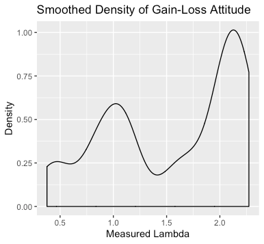
#First, plot a kernel smoothed density of the Lambda.
library(ggplot2)
density_plot<-ggplot(orig_data, aes(Measured_Lambda)) + geom_density()+
  labs(x="Measured Lambda", y="Density", title = "Smoothed Density of Gain-Loss Attitude")


#Finally, run the regression of interest.
interaction_reg=lm(VoluntaryExchange~Treatment+Measured_Lambda+(Treatment*Measured_Lambda), data = orig_data)
summary(interaction_reg)
library("stargazer")
stargazer(interaction_reg, title="MSL Interaction Regression",
          align=TRUE, dep.var.labels=c("Exchange (=1)"),
          covariate.labels=c("Treatment","$\\hat{\\lambda}_i$",
                             "$\\hat{\\lambda}_i \\times$ Treatment"),
          omit.stat=c("LL","ser", "aic", "bic"), no.space=TRUE)

Lambda_Dist_Blog


MSL_Table

Sources:
Goette, Lorenz, Thomas Graeber, Alexandre Kellogg, and Charles Sprenger (2018). “Heterogeneity of Gain-Loss Attitudes and Expectations-Based Reference Points”.
Kőszegi, Botond and Matthew Rabin (2006). “A model of reference-dependent preferences”. In: The Quarterly Journal of Economics, pp. 1133–1165.
Kőszegi, Botond and Matthew Rabin (2007). “Reference-Dependent Risk Attitudes.” In: American Economic Review (4): 1047–73.


Power Analysis Code (Python)

Introduction

A fundamental part of experimental economic research is writing pre-analysis plans, which serve as a commitment device for the hypotheses we wish to test and the number of participants we aim to recruit. In outlining the specific questions we are seeking to answer with a specific sample size, we can reassure future readers that the findings we describe are not a coincidence which we stumbled upon as we analyzed our data, lending increased credibility to the experimental results. The following sections describe one particular (preliminary) exercise conducted in the pre-analysis plan for a working paper of mine, Campos et al (2019).

Our project is a natural follow-up to a submitted project of mine, Goette et al (2019), in which we derive and test comparative static predictions of the KR model in the endowment effect context with heterogeneous gain-loss types. Specifically, we consider two types of agents: loss averse and gain loving. Loss averse individuals, roughly speaking, are defined as those who would accept a 50-50 gamble of +$10+x, -$10 for x>0; intuitively, these agents dislike losses around a reference point (assumed 0 here) more than equal sized gains, and would thus need to be compensated with a bigger payoff to accept the possibility of a $10 loss. The larger the x before they accept, the more loss averse. Gain lovers, in the same rough terms, would actually accept gambles where x<0 because, intuitively, they enjoy the surprise of the lottery, and enjoy gains above the reference point more than commensurate losses.

In Goette et al (2019), we show that lab participants previously measured to be gain loving vs loss averse respond quite differently to a treatment that is commonly used to test the KR model. Importantly, prior analysis of these types has tended to ignore the heterogeneity and test the treatment assuming that people are loss averse on average. Although this is empirically true, the 15-30% of gain lovers have an outsized role in aggregate treatment effects, which we uncover in our paper. The pre-analysis exercise described below applies this same experimental framework to a different domain, to explore whether these gain-loss classifications predict behavior in the real effort setting.

Power Analysis Overview and Code

Before we run our experiments in this new domain, we want to be sure that the theoretical predictions yield interesting, testable implications that can be measured with reasonable sample sizes. To get a feel for this, we run simulations on bootstrapped data, allowing us to recover expected treatment effect sizes under heterogeneous populations. From the data in Goette et al (2019), we obtain a distribution of gain-loss attitudes measured in a lab population — which we assume to be representative despite the domain change. From Augenblick and Rabin (2018), we obtain MLE estimates of the cost of effort function under a particular functional form assumption, using the same task as we will in this experiment (see Table 1 for parameter estimates).  With these distributions of parameters in hand, we have all the requisite information to generate simulated behavior under the KR model, specifically the CPE assumption.

For a range of sample sizes, we bootstrap from these distributions and generate simulated behavior, which we subsequently feed into our regression of interest. For each of the sample sizes we consider, we store the estimated regression coefficient as well as the minimum detectable effect size (approximated by 2.8*SE(coef) as in Page 16 of these JPAL slides), which we ultimately plot against the bootstrapped sample. This plot helps inform us of what types of effect sizes we can reject at different sample sizes; by examining our simulated effect sizes, we are able to map the results and determine the number of participants we require.

Note that there are a number of simplifications in this code, and the final sample size will be determined using a slightly different procedure. Specifically, the analysis herein assumes we know the gain-loss value (lambda), whereas in our study, we will estimate it from experimental data. Because this introduces additional noise, we expect attenuation bias in our parameter estimates. This, and other details that were skipped over, will be discussed at length in the pre analysis plan; as soon as it is posted, I will link to it.

This Python code implements the aforementioned procedure, generating a preliminary MDE curve.

'''
Code Overview: Using data from Goette et al (2019) and Augenblick and Rabin (2019),
we bootstrap a distribution of gain-loss and cost of effort function parameters to
conduct a power analysis on our experimental hypothesis. Ultimately, we hope to
determine the requisite sample size to test our coefficient of interest with 80%
power at the 5% two-sided level.

Author: Alex Kellogg
'''

#Import required modules for the ensuing analysis
import numpy as np
import pandas as pd
import matplotlib.pyplot as plt
import statsmodels.formula.api as sm

'''
We assume the distribution of gain-loss attitudes follows that in Goette et al (2019)
for  this analysis. This data was estimated via MLE in a prior project, and is
generally representative of the experimentally measured distributions throughout the
literature.
'''

#Read in the relevant columns from full Goette et al (2019) lab data
ggks_dataset=pd.read_csv("dir/pooled_data.csv", usecols=['stage1_lambda','structla'])

'''
Because our task is adopted from Augenblick and Rabin (2019), who have prior
MLE estimates of the cost of effort function given their assumed functional
form, we opt to model effort costs in the form below. This allows us to introduce
heterogeneity in a rigorous manner to both cost of effort and gain-loss attitudes.
'''

def cost_of_effort(e, c_slope, c_curv):
    '''
    :param e: Effort, or the number of tasks (b/w 0 and 100).
    :param c_slope: Slope parameter, normalizing tasks to dollar costs.
    :param c_curv: Curvature parameter determining convexity of cost function.
    :return: (Negative of) Utility from completing e tasks.
    '''
    return (1/(c_slope*c_curv))*((e+10)**c_curv)

'''
We assume individual utility follows KR06 CPE, so that there is no gains/losses
in the effort domain as the number of tasks are preselected, but uncertainty
in wages yields gain-loss comparisons against reference points. Specifically,
each feasible ex-ante outcome is compared to the others, weighted by their a-priori
likelihood.

'''
def cpe_utils(e, c_slope, c_curv, wage, fixed, lam):
    '''

    :param e: The number of tasks considered.
    :param c_slope: Slope parameter, normalizing tasks to dollar costs.
    :param c_curv: Curvature parameter determining convexity of cost function.
    :param wage: Piece-rate (per task) rate of payment.
    :param fixed: Outside option, which is earned regardless of effort with 50%.
    :param lam: Gain-loss Attitude parameter, lam>1 implies loss aversion.
    :return: KR06 CPE utility of working e tasks given the preference parameters and wage rates.
    '''

    return 0.5*e*wage+0.5*fixed-0.5*(lam-1)*abs(fixed-wage*e)-cost_of_effort(e,c_slope,c_curv)

'''
Unfortunately, there is no closed form solution to the problem of optimal effort with
fixed vs piece-rate wages. Thus, to determine the optimal utility given the parameters,
we conduct a grid search over the possible values of effort, which can range between 0
and 100 tasks. The alternative to a grid search is a series of elseif conditions to
determine how the Marginal Benefit and Marginal Cost curves relate to each other, but
the number of checks is extensive and thus the computational cost of the grid search
outweighs the speed but increased error rate of the checklist approach.
'''

#Loop over the possible task choices for the agent given the parameters, and store the optimal
def optimal_effort_solver(c_slope, c_curv, wage, fixed, lam):
    '''
    :param c_slope: Slope parameter, normalizing tasks to dollar costs.
    :param c_curv: Curvature parameter determining convexity of cost function.
    :param wage: Piece-rate (per task) rate of payment.
    :param fixed: Outside option, which is earned regardless of effort with 50%.
    :param lam: Gain-loss Attitude parameter, lam>1 implies loss aversion.
    :return: The number of tasks that yields maximum CPE Utils.
    '''
    effort_space = np.arange(0, 100.1, 0.1)
    utils_vec=[]
    for a in effort_space:
        tempU= cpe_utils(a, c_slope, c_curv, wage, fixed, lam)
        utils_vec.append(tempU)
    utils_vec = np.asarray(utils_vec)
    max_ind = np.argmax(utils_vec)
    return effort_space[max_ind]

#Define a function the computes the between subjects interaction regression.
def treatment_effect_bootstrapped_between_lambda(data):
    '''
    :param data: Dataframe containing the relevant variables for the regression specification.
    :return: Regression Result.
    '''

    #generate a new effort variable that captures only the relevant effort given treatment
    data['Effort']=data['Treatment']*data['Effort_Choice_Hi_Fixed']+(1-data['Treatment'])*data['Effort_Choice_Low_Fixed']

    data['Interaction']=data['Treatment']*data['Lambda']

    result = sm.ols(formula="Effort ~Treatment+Lambda+Interaction", data=data).fit()
    return result

#Create a function to plot the Minimum Detectable Effect size
def mde_plotter(n_list, mde_list):
    '''

    :param n_list: np.array of the sample sizes we considered in the MDE analysis.
    :param mde_list: List of the mde's generated in the analysis.
    :return: Plot the MDE for each sample size.
    '''
    mde_list=np.asarray(mde_list)
    plt.plot(n_list,mde_list)
    plt.xlabel('Bootstrapped N')
    plt.ylabel('MDE')
    plt.show()

#Set up the parameters for our MDE analysis loop.
bootstrap_N_list=np.arange(50,1000,50)
bootstrap_MDE=[]
bootstrap_te=[]

'''
Iterate over each of the sample sizes and compute the MDE at that sample size.
To do so, we will sample bootstrap_N gain-loss, cost slope (constant here),
and cost curvature parameters from their assumed distributions, based on prior work.
We take this sample to be our experimental subject pool, and simulate the decisions
we would observe from these subjects if they decided according to KR CPE. We then run
our interaction specification on our full sample and record the parameter estimate for
coefficient of interest, as well as the mde, which is approximated by 2.8*SE(beta).
'''
for bootstrap_N in bootstrap_N_list:
    #sample lambdas with replacement from the empirical distribution to create our own distribution
    id = np.random.choice(np.arange(len(ggks_dataset.stage1_lambda)), bootstrap_N, replace=True)
    sampled_lambda = np.asarray(ggks_dataset.stage1_lambda[id])
    sampled_structla = np.asarray(ggks_dataset.structla[id])

    #for the cost function, we borrow numbers from Table 1 (pg 29) in AR19 assuming the large sample properties of MLE.
    #that is, we take the estimated MLE and associated sd to be distributed normally, and draw from them.
    # cost slope represents phi in the AR cost function.
    cost_slope = [724] * bootstrap_N
    # cost curvature represents gamma.
    cost_curvature = np.random.normal(2.138, 0.692, size=bootstrap_N)

    #To cut the computation in half, we solve for the optimal effort in the condition for which this simulant will ultimately wind up.
#This is a between subjects regression, so it is unaffected.
    treatment_assignment=np.random.randint(2, size=bootstrap_N)

    effort_choices_l=[]
    effort_choices_h=[]
    for i in np.arange(0,bootstrap_N):
        if treatment_assignment[i]==0:
            effort_choices_l.append(optimal_effort_solver(cost_slope[i], cost_curvature[i], 0.25, 5, sampled_lambda[i]))
            effort_choices_h.append(-1)
        else:
            effort_choices_l.append(-1)
            effort_choices_h.append(optimal_effort_solver(cost_slope[i], cost_curvature[i],0.25,20,sampled_lambda[i]))

    #Define the dataframe to feed into the regression function.
    df_cols={
        'Effort_Choice_Low_Fixed':list(map(float, np.asarray(effort_choices_l))),
        'Effort_Choice_Hi_Fixed':list(map(float, np.asarray(effort_choices_h))),
        'Lambda': sampled_lambda,
        'Structla': sampled_structla,
        'Cost_Slope': cost_slope,
        'Cost_Curvature': cost_curvature,
        'Treatment': treatment_assignment
    }
    bootstapped_data = pd.DataFrame(df_cols)

    reg_results=treatment_effect_bootstrapped_between_lambda(bootstapped_data)
    bootstrap_MDE.append(reg_results.bse[3]*2.8)
    bootstrap_te.append(reg_results.params[3])

#plot the MDE curve
mde_plotter(bootstrap_N_list,bootstrap_MDE)

The resulting plot is displayed below. Our median effect size is roughly 15 tasks in this particular simulation, which would suggest a sample of about 400 to be sufficient.

mde_plot

Sources:
Augenblick, Ned and Matthew Rabin (2018). “An Experiment on Time Preference and Misprediction in Unpleasant Tasks”.
Goette, Lorenz, Thomas Graeber, Alexandre Kellogg, and Charles Sprenger (2018). “Het- erogeneity of Gain-Loss Attitudes and Expectations-Based Reference Points”.
Kőszegi, Botond and Matthew Rabin (2006). “A model of reference-dependent preferences”. In: The Quarterly Journal of Economics, pp. 1133–1165.
Kőszegi, Botond and Matthew Rabin (2007). “Reference-Dependent Risk Attitudes.” In: American Economic Review (4): 1047–73.

Understanding Workers’ Valuations of Various Amenities: A Summary of Mas and Pallais (Forthcoming)

The following summary and thoughts on Mas and Pallais (Forthcoming in the AER, 2017) is taken in part from a report I put together for a course in labor economics. In this study, the authors present their results from the first large-scale field experiment attempting to elicit workers’ valuations of specific amenities (e.g. working from home, flexible hours, flexible scheduling). The paper provides a critical foundation for future research in understanding workers’ preferences over a variety of work arrangements that are commonly offered by employers.

Overview of Mas and Pallais (forthcoming AER 2017)

To gather data on workers’ willingness to pay (WTP) for different amenities, the authors recruit staffers for a national call center for the purpose of administering surveys unrelated to this project. Advertisements were posted online in 68 large metro areas, and potential applicants were able to click-through into the application, wherein they (optionally) listed their race, ethnicity, and gender. Next, the applicants specified which of two job opportunities they would prefer: the “baseline” job at a specified wage or a “treatment” job at a potentially different wage. The main treatments included: work from home (ability to work from home, Mon-Fri 9am-5pm), flexible scheduling (ability to choose how to allocate 40 hours per week), flexible hours (ability to choose the amount of hours up to 40 hours per week), and employer discretion (the employer sets your schedule every week with a one week notice, and work times can include weeknights or weekends).

In order to estimate the distribution of worker’s WTP, the authors randomly selected wages and assigned them to one of the two jobs. For each pair the applicant saw, one job always had the maximum wage of $16 per hour (or 19, depending randomly on the city) while the other had a wage within 5 dollars of the maximum wage (+/- $0.25, $0.50, $0.75, … , $2.75, $3, $4,or $5). The applicants were told that this choice would not affect their hiring decision, and would only be seen by the employer after a hiring decision had been made. Thus, this field experiment is a between-subjects design with around 7,000 applicants – 150 of whom have been offered a job with the “best amenities” (maximum wage that applicant saw, the ability to work from home, and scheduling flexibility).

From this experiment, the authors learned that the majority of workers do not value scheduling flexibility (setting the total number of hours or setting the schedule for 40 hours per week), but, on average, workers were willing to take an 8% pay cut to work from home (see Fig 4 reproduced from the paper below). Not surprisingly, workers had a strong distaste for the employer discretion job offer: the average worker was willing to take a 20% lower wage to avoid these jobs, and close to 40% of applicants preferred the baseline job even if the employer discretion offered a 25% higher wage. Although these average effects are important, the amount of heterogeneity in valuations was striking and leaves room for further investigation. For more results, consult Figures 2-6 from Mas and Pallais (Forthcoming in the AER, 2017).

Mas Fig 4
Reproduced from Mas and Pallais (Forthcoming).

As with all field experiments, external validity is a natural concern; do these results only apply to the subsample of applicants observed in the data (people who would apply for a position as a survey administrator), or do they generalize to the population at large? To address this issue, the authors presented numerous supplemental experiments as well as additional empirical work. In particular, to obtain a more nationally representative sample (as opposed to the self-selected sample of phone survey applicants), the authors asked essentially the same questions (this time, completely unincentivized) to participants in the Understanding America Study (UAS) (a nationally representative Internet panel conducted by USC, with around 6,000 total households). The results from this alternative data source were consistent with the field experiment. Since these specific questions are hypothetical, however, the robustness of these results isn’t totally assured; nevertheless, the evidence that more nationally representative samples of workers had similar valuations (as well as a number of robustness checks included in the full paper) increases my confidence in their results.

Finally, the authors do some preliminary exploration of workers’ heterogeneity in WTP for the various arrangements. In particular, using the UAS (where they have more data on covariates), they determine that workers tend to sort into their preferred arrangements (those with the highest WTP for an amenity tend to pay for it), and find that mothers of young children value the ability to work from home twice as much as men.

Remarks

Overall, this paper provides one of the first in depth analyses of worker’s valuations for different job arrangements. Although some literature exists on this topic, much of it is imprecisely estimated, which makes this field experiment all the more valuable as it presents a novel approach to an old question. Moreover, the authors are very thorough in their work, providing a multitude of robustness checks for each of their major findings. Finally, the nature of the data collection is very rich as it allows readers access to the raw WTP averages, from which a distribution can be estimated. I perceive these to be the major strengths of this paper.

As with all papers, however, there are some shortcomings. The main issue, as I see it, is the incentive structure behind the field experiment: the results would be stronger if the hired applicants received their actual choice between baseline and “treatment” instead of the highest wage and most liberally arranged job. In this way, the authors break from a traditional field experiment, and produce more of what might be called a “survey experiment in the field”. Luckily, the applicants were very unlikely to know the details of the final job offer (the authors offered each successful applicant a job with the “best amenities”), so there is almost certainly no inadvertent impact on the workers’ answers.

I’m also curious why they chose the occupation they did: although perhaps the authors expected lower skilled workers would value the amenities more, I suspect that college graduates might actually be willing to pay much more for these options. It would be interesting to see if that is the case, since it seems (from the supply side) that companies like Google or Facebook offer many of these amenities and flexibilities.

In any case, I am looking forward to learning more about the heterogeneity of valuations for amenities. In particular, I’m curious about the points of excess mass that the authors discovered in the Cumulative Distribution Function of workers’ WTP. Since the CDFs in the figures above represent the proportion of workers who are willing to pay $X or less for the amenity, the large spikes at certain prices are perhaps indicative of some behavioral phenomena. For example, these spikes could potentially represent the price associated with the uncertainty of switching amenities away from the default, the mental cost of making a decision, or a reference point of some sort.

Ultimately, I believe there are many interesting questions to be asked about all of the findings presented in this paper, and expect to see this literature rapidly expand in the coming years.

Sources

Mas A, Pallais AValuing Alternative Work Arrangements. American Economic Review. Forthcoming

Economics of Terrorism

This post is based on a recent lecture by Eli Berman, which was based in large part on the paper “Sect, Subsidy, and Sacrifice: An Economist’s View of Ultra-Orthodox Jews“.

Much of human behavior can be analyzed through the lens of economics, including religious practice. Adam Smith had some thoughts on the matter in “An Inquiry into the Nature and Causes of the Wealth of Nations“, where he argued that competition among religious sects would lead to less political clout for the church and harder working church officials.

However, not much progress had been made in the ensuing 216 years. Eventually, Laurence Iannaccone picked up the mantle in 1992 and revolutionized the economics of religion by modeling religion as a club good — meaning that it is non-rival but excludable. That is, multiple people can practice the same religion at the same time, but individuals can be forbidden from practicing within a certain sect or church (e.g. through ex-communication). Thus, religion invites the free-rider problem, wherein certain practitioners don’t contribute to the religious experience but still get benefits.

At this point, we turn our attention to Laurence Iannaccone’s groundbreaking work. According to his model, free-riding agents diminish the experience of the entire group, and would ideally (for the sect) be restricted from practicing in the future. That is to say, an ideal sect — from a group member’s perspective — is mostly filled with people who will devoted their time to the practice. This way, each of the members is willing to spend time taking care of the others within the sect based on anticipated reciprocity, providing a sort of insurance for members. Berman described an ideal sects in terms of an ideal study group: you want members to have read the papers you will be discussing, so you want to incentivize members to spend their time reading. This can be done by limiting study partners’ outside options (e.g. no drinking on weekends) or by expelling members who don’t contribute.

People who have relatively low wages (and thus a lower opportunity cost of time) are theoretically more willing to devote their time to religion — a hypothesis that is empirically validated (see this paper for more detailed proof). Thus, under this model, churches might want to attract low wage individuals in order to provide a better experience for the group as a whole. (Note that attracting richer individuals who substitute time for donations also plays a role in more complicated models, but recruiting lower wage individuals will nevertheless increase the benefits to joining a particular sect.) Since the church cannot observe their practitioners’ wages, how can they exclude high wage people masquerading as low wage people? In terms of the study group analogy, how can the members tell if a potential new recruit is willing to put in the time and do the reading?

It turns out that this is a signaling problem; thus the church thus has to design incentives such that low wage and high wage people self select (or separate) in equilibrium.  There are two ways a church goes about this: prohibitions and sacrifices. Strict dress codes, the barring of alcohol/caffeine/sex, and time commitments are examples of prohibitions and sacrifices imposed by some religions. Together, these tools can be used to weed out high wage earners who value their time relatively more. That is, high earners are more likely to prefer working more and forgoing these particular restrictions as opposed to joining the sect, dedicating a substantial amount of time, and following the strict rituals. Bringing back the analogy of the study group, setting up meetings on Friday or Saturday nights (thereby increasing the costs of going out drinking) might increase the likelihood that members read prior to meetings, thereby making meetings more productive.

Connecting the economics of religion to terrorism, Berman and Iannaccone argue in “Religious Extremism: The Good, the Bad, and the Deadly” that the aforementioned religious organizational structure is a major contributor to violent terrorism, more so than a belief in afterlife rewards or a specific theology.  To develop this intuition, consider a violent organization intent on conducting an act of terrorism. In order to succeed, the group must plan the attack, which requires coordination among the members. However, coordination invites the threat of defection, since any member could turn on the group and receive a large reward. How can these terrorist organizations reduce the likelihood of defection?

Just like the aforementioned radical sects, these violent organizations will seek members who are willing to sacrifice their time and succumb to prohibitions. In other words, radical sects provide a ready-made pool of ideal participants from the point of view of these terrorist groups; the core members of these sects are a self-selected pool of highly committed individuals with a low opportunity cost of time who are willing to endure various prohibitions to be part of the club. This idea is reflected in interviews of jailed terrorists, who tend to join their respective violent organizations for many of the same reasons that people join certain religions or political parties.

To test this idea, one can compare the violent behaviors of different sects within an overarching theology. Berman and Laitin’s “Religion, terrorism and public goods: Testing the club model” provides us with just this empirical test; their findings confirm that members of religious groups that require more sacrifices and prohibitive behaviors attempt significantly more attacks (and are more effective) than others with similar, less prohibitive beliefs.

So, where do we go from here? Since most of the violent organizations come from relatively impoverished countries, Eli Berman suggests that increasing access to public goods and property rights is fundamental. Providing more public goods will lead to less demand for the “clubs” that are religious sects and violent terrorist organizations, since would be members would have more alternatives to receive the benefits that these groups are relied upon to provide. In addition, improved property rights and contract enforcement would partially solve some of the missing market problems that incentivize people to join radical sects; if people don’t have to worry about losing their food supply or their home, joining a radical sect is relatively more costly. Finally, since all models are imperfect descriptions of reality, social scientists should continue to focus on these topics so that we may derive better policy going forward.


If you’re interested in learning more about this, I suggest reading the sources below or visiting Eli and Laurence’s websites to find some cool papers.

Sources:

Berman, Eli, “Sect, Subsidy and Sacrifice: An Economist’s View of Ultra-Orthodox Jews,” Quarterly Journal of Economics, August 2000

Berman, Eli, and David D. Laitin. “Religion, Terrorism and Public Goods: Testing the Club Model.” Journal of Public Economics 92.10-11 (2008): 1942-967.

Iannaccone, Laurence R (1998) “Introduction to the Economics of Religion,” Journal of Economic Literature, 36, pp. 1465-1496.

Iannaccone, Laurence R. “Sacrifice and Stigma: Reducing Free-riding in Cults, Communes, and Other Collectives.” Journal of Political Economy 100.2 (1992): 271-91.

Iannaccone, Laurence R., and Eli Berman. “Religious Extremism: The Good, the Bad, and the Deadly.” Public Choice 128.1-2 (2006): 109-29.

Post, Jerrold, Ehud Sprinzak, and Laurita Denny. “The Terrorists in Their Own Words: Interviews with 35 Incarcerated Middle Eastern Terrorists∗∗This Research Was Conducted with the Support of the Smith Richardson Foundation.” Terrorism and Political Violence 15.1 (2003): 171-84.

Smith, Adam, An Inquiry into the Nature and Causes of the Wealth of Nations (Reprint of 1776 version) Modern Library: New York; 1965. Book V, Chapter I, Part III, Article III “Religious
Institutions.


Thoughts on the Federal Reserve vs Trump

Over the last few weeks, the Federal Reserve has come under criticism from Mr. Trump, the Republican presidential nominee. Although Mr. Trump is not known for his policy or economic expertise, he claims that the Fed’s refusal to raise interest rates is motivated by political considerations, bemoaning that the Fed “made the political decision every single time.” In Fed Governor Lael Brainard’s speech The New Normal and What It Means For Monetary Policy, she provides more than enough evidence that the Federal Reserve is in fact acting in the interest of both the US and global economy.

In particular, Governor Brainard correctly points out that the policy tools the Fed has at its disposal are asymmetric with the federal funds rate so low; here are her exact words,

“In today’s new normal, the costs to the economy of greater-than-expected strength in demand are likely to be lower than the costs of significant unexpected weakness. In the case of unexpected strength, we have well-tried and tested tools and ample policy space in which to react. Moreover, because of Phillips curve flattening, the possibility of remaining labor market slack, the likely substantial response of the exchange rate and its depressing effect on inflation, the low neutral rate, and the fact that inflation expectations are well anchored to the upside, the response of inflation to unexpected strength in demand will likely be modest and gradual, requiring a correspondingly moderate policy response and implying relatively slight costs to the economy. In the face of an adverse shock, however, our conventional policy toolkit is more limited, and thus the risk of being unable to adequately respond to unexpected weakness is greater.”


In other words, Gov. Brainard is saying that the Federal Reserve is highly susceptible to a new recession. Because interest rates are low, one might worry about inflationary pressures (though that has yet to be an issue, with inflation at around 1%). That is why some (Mr. Trump included) want the Fed to raise rates. However, Gov. Brainard is arguing that the Fed is well-equipped to deal with rising inflation. On the other hand, because rates are already so low, there are potentially grave risks associated with increasing the federal funds rate. Specifically, the economy may tighten too much leading to a recession, but the Fed will be unable to effectively combat that recession by lowering interest rates since they are already so low. Let’s delve deeper into the two sides, to get a more nuanced understanding of the argument.

The potential issue with a “greater-than-expected strength in demand” (think consumers suddenly buying more goods, because the cost of borrowing is so low) is rising inflation, which Brainard explains may be tempered as a result of a variety of conditions, including:

  1. The flattening of the Phillips Curve, meaning if GDP goes over its natural rate (as it might with stronger demand than expected), the rate at which inflation increases will be subdued (relative to the past)
  2. The slackness of the labor market, so that GDP may still be below its natural rate (not at full capacity yet, essentially) so a strong demand increase would not have as large an impact on inflation.

Because of these and the other listed factors in the article, the Fed is not too preoccupied by the possibility of unexpectedly strong demand. Moreover, if such a shock were to occur and increase inflationary pressures by too much, the Fed’s most likely response – tightening the monetary reigns by increasing rates – is still very much in play. All this to say, keeping rates too low for too long is not a big deal, as a surge in demand can be managed with relative ease.

On the flip side, Gov. Brainard admits that “In the face of an adverse shock, however, our conventional policy toolkit is more limited, and thus the risk of being unable to adequately respond to unexpected weakness is greater.” If the Fed raised the rates – acting as Mr. Trump and others have suggested – demand in the economy would naturally tighten (the cost of borrowing is now higher, so people will tend to save more if the rates increase). If the economy tightens too much, a recession will follow. The most effective way for the Fed to fight recessions using monetary policy is to lower the interest rates. However, since the rates are already so close to zero, the Fed will not have much room to act, thereby leaving it relatively incapable of handling an adverse shock in demand. Thus, the cost of increasing the rates is in part the risk of causing a hard-to-fight recession.

Based on this analysis, it’s evident that the precautionary strategy of slowly raising rates is economically well-founded. So next time you hear Mr. Trump say that the Fed is acting purely politically, ignore him.


Thanks to Alex Weiss for discussing the speech with me, and providing valuable intuition.

The Year of the Underdog Continues at Euro 2016

Yet again, 2016 has witnessed an upset in a major sporting event. The 73-9 Warriors fell to the Cavs. Leceister City won the Premier League. Novak Djokovic was eliminated in the early rounds of Wimbledon, ending his 30 game win streak in Majors. Argentina fell to Chile (though cynics will claim this was to be expected considering Argentina is 0 for 6 in major finals since 2000). Now France, the host of the Euro Cup, has been defeated by Portugal.

The game, much like the majority of the tournament, was slow and disappointing throughout. Cristiano Ronaldo was injured early on, and was crying while taken off the field by a stretcher in the 25th minute. France pushed hard in the opening minutes in an effort resembling the semi-final versus Germany, but wound up slowing down the pace thereafter and were content with maintaining possession around Portugal’s box. Portugal played as they had all tournament, offering very little offensively and wearing down the opposition by keeping possession in their own half. Griezmann and Gignac had two excellent chances, the former was headed right over the open goal and the latter clattered against the post and out; for Portugal, Quaresma nearly drilled a bicycle kick past Lloris. Though I can’t speak for everyone, I doubt either team’s fan base was particularly content with the play during regulation.

In extra-time, the players picked up right where they left off, though mental errors and physical exhaustion were much more prevalent for both sides. In the 107th minute, the game took a drastic turn when Koscielny was wrongly carded for a hand ball. The Portuguese nearly capitalized on the free-kick from 25 or so yards out, hitting the crossbar, and nearly giving the French a heart-attack. Just two minutes later Eder drilled a 25 yard shot low to Lloris right, and the rest – as they say – is history. You can see the goal here, for reference.

As we’ve seen many times before and we will see many times to come, the better team lost today. France dominated possession for large parts of the game, but were unable to breach Portugal’s bunkered down defense; the few clear cut chances they got were either wasted or saved by Rui Patricio. Portugal, for their part, played an ugly but tactically sound game of soccer and were ultimately able to convert one of their 3 shots on goal. Though the game certainly won’t be celebrated by critics and fans alike, it emphasizes a mental shift by (usually weaker) teams to a defensive brand of soccer – the sort that helped propel Chelsea to the Premier League title last year.

In retrospect, Koscielny should’ve have taken Eder down before he had the chance to shoot; he certainly would’ve received a second yellow card, but a 10 men France likely could have let the game ease into penalty kicks. His decision making, though instantaneous, was clouded by the prior call wherein referee Mark Clattenburg erroneously gave the French defender a yellow card. Upon replay, it’s clear that the ball went off of Eder’s hand and this unfortunate (but understandable) miscall wound up costing France a goal. Perhaps a review system in soccer would have led to a different outcome, but that’s a topic for another day. In any case, it’s hard to win when you don’t score a goal.


What Matters More: Regular Season or Playoffs?

As a Sharks fan throughout most of my childhood, I was terribly disappointed when the Sharks won the President’s Trophy in the 2008-9 season and were prematurely ousted from the Stanley Cup Playoffs. How can a team that cruises by all of its opponents in the regular season suddenly collapse in the playoffs, and “waste” the entire season? The amazing run of the 16-0 Patriots was similarly disregarded after they fell to the New York Giants in the Super Bowl, as was the 116-46 record of the 2001 Mariners, and many other teams before them. This year, I had the good fortune of watching the Golden State Warriors finish off the greatest regular season in history. Who could’ve imagined this team would lose 9 games the entire 82 game long season? But again, playoff hysteria gripped the nation and now NBA fans and critics around the country are discrediting the marvelous feat this team accomplished. “73 wins means nothing without a ring” I hear, or “Greatness is defined in June”. To me, that’s nonsense.

If we look to professional soccer leagues in Europe, the EPL or La Liga as the leading examples, there are different types of greatness: international cups (Europa, Champions Leauge), Domestic Cups (FA Cup, Copa del Rey), and winning the league itself. Each of these three types of competitions offer teams a different challenge. On a given day any team could win a single elimination game, while the double round-robin system requires tactical mastery. Upsets are expected in these tournaments and are a major reason these competitions draw so much excitement. Over a long season however, the cream rises to the top, and so a different sort of champion is born. Regardless of the system used to crown a winner, each is valued about as much as the next. That is to say, winning the league is a huge deal.

The point of a long season is to diminish the impact of random win streaks on the ultimate league rank. Playoffs, on the other hand, reward teams that find their groove in a one-month span, thus luck plays a much larger role in determining playoff champions (best of seven series are better in that regard than the NFL, or even the MLB opening rounds). Sure, these victories should be celebrated, but they shouldn’t be legacy defining moments.

Think of Leceister in the EPL this past year and their media reception around December, when they were top of the table. Everyone believed them to be having a stretch of unsustainably good form, to have had easy match-ups with weakened sides, and to fall to mid-table within a two months. Yet they held strong, remained atop the league, and rode the long season down to its glorious end. Leceister are champions because they fought through 38 arduous games, and led the league when the final whistle blew. They are champions because they weathered storms, they fought back from losing streaks, and they remained consistently better than their opponents in the long run. Barcelona, who are certainly not underdogs in La Liga, also came out of the long season victorious. Though they were unable to repeat the Treble (league, domestic cup, and international cup champions), their fans were nonetheless elated when they won the league. So why is it that the Warriors, who tore apart the NBA in the regular season, are dismissed and chided for their playoff performance?

It must have something to do with American sports culture, and American sports. The simplest way to see that is to compare the MLS to the EPL or La Liga or Ligue 1. In the EPL for instance, there is one table that ranks all teams and there are a couple different tournaments that span nearly the entire season. The MLS instead opts for an Eastern and a Western conference, similar season long tournaments, and finally a post-season playoff within each division that culminates in an East vs West final. Though both the MLS and the EPL have domestic competitions as well as a league winner, neither of these two pieces of silverware matter much to MLS fans. In the US, only the MLS Cup victor gets their parade (whereas Arsenal paraded their winning of the FA Cup in 2015, for example).

Though I can only speculate as to the reasons Americans value playoffs so much, I imagine it has something to do with the branding and the set-up of the league. With regards to branding I am specifically talking about linguistics; naming the winner of a tournament “Champions” makes the tournament more significant, especially when the winner of the regular season is usually deemed “Winners of XYZ Cup” or not even recognized. In addition, the fact that playoffs come at the end of the season gives fans a sense of closure; when a team wins the very last game of the playoffs, it feels like they’ve won everything, like they are indeed the one and only champions. Finally, it could have something to do with the length of the season – though this predominantly applies to the MLB, NBA, and NHL. When a season consists of more than 80 games, most fans don’t watch every game. Thus, it is more difficult to sell advertisements especially when the match-up is a “Garbage Bowl”. However, playoffs provide an ideal revenue-making opportunity for the league: a best of 7 series where every game matters, so that fans have no choice but to stay glued to their television. By the time the Conference Finals and the Finals arrive, fans and non-fans alike tend to tune-in to see who the champion will be. Evidently, this is an excellent way to reap profits and since the league managers understand this, they hype up the playoffs any chance they get.

Although playoff culture is deeply ingrained in American sports, it is too prone to hot/cold streaks to be the lone determinant of greatness. Playoffs are a fun and exciting time to be a sports fan as they provide a shorter, more intense version of the prior months-long season. The winners of these tournaments certainly earn their right to celebrate. But Hall of Fame players (like Allen Iverson, Charles Barkley, Ken Griffey Jr, Alex Ovechkin, Kevin Durant, etc) should not be looked down upon for failing to win the playoffs. Consistent greatness, in the form of an incredible regular season run or a player’s career-long achievements, should be celebrated and valued equally in their own right. If playoffs really are the only relevant factor in determining greatness and legacies, why bother playing a regular season?